Stellar Module#
This module include general functions to work with stars
Stellar cluster#
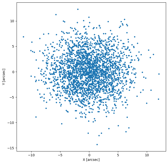
In the following example we generate a young star cluster with a core radius r_c=1 pc, M=1000 Msun and located in the LMC (d=50kpc)
import numpy as np
from scopesim_templates.stellar import cluster

src = cluster(mass=1E3, distance=50000, core_radius=1)
/home/docs/checkouts/readthedocs.org/user_builds/scopesim-templates/envs/latest/lib/python3.11/site-packages/tqdm/auto.py:21: TqdmWarning: IProgress not found. Please update jupyter and ipywidgets. See https://ipywidgets.readthedocs.io/en/stable/user_install.html
  from .autonotebook import tqdm as notebook_tqdm
imf - sample_imf: Setting maximum allowed mass to 1000
imf - sample_imf: Loop 0 added 1.09e+03 Msun to previous total of 0.00e+00 Msun
Downloading file 'pickles98_full.fits' from 'https://scopesim.univie.ac.at/pyckles/pickles98_full.fits' to '/home/docs/.astar/pyckles'.
Downloading file 'filter_systems/etc/index.yml' from 'https://scopesim.univie.ac.at/spextra/database/filter_systems/etc/index.yml' to '/home/docs/.spextra_cache'.
0%| | 0.00/609 [00:00<?, ?B/s]
0%| | 0.00/609 [00:00<?, ?B/s]
100%|██████████████████████████████████████████| 609/609 [00:00<00:00, 387kB/s]
Downloading file 'filter_systems/etc/V.dat' from 'https://scopesim.univie.ac.at/spextra/database/filter_systems/etc/V.dat' to '/home/docs/.spextra_cache'.
0%| | 0.00/3.18k [00:00<?, ?B/s]
0%| | 0.00/3.18k [00:00<?, ?B/s]
100%|█████████████████████████████████████| 3.18k/3.18k [00:00<00:00, 2.22MB/s]
Downloading file 'libraries/ref/index.yml' from 'https://scopesim.univie.ac.at/spextra/database/libraries/ref/index.yml' to '/home/docs/.spextra_cache'.
0%| | 0.00/576 [00:00<?, ?B/s]
0%| | 0.00/576 [00:00<?, ?B/s]
100%|██████████████████████████████████████████| 576/576 [00:00<00:00, 404kB/s]
Downloading file 'libraries/ref/vega.fits' from 'https://scopesim.univie.ac.at/spextra/database/libraries/ref/vega.fits' to '/home/docs/.spextra_cache'.
0%| | 0.00/276k [00:00<?, ?B/s]
5%|██ | 14.3k/276k [00:00<00:02, 121kB/s]
17%|██████▌ | 46.1k/276k [00:00<00:01, 206kB/s]
24%|█████████▌ | 67.6k/276k [00:00<00:01, 193kB/s]
36%|██████████████▌ | 100k/276k [00:00<00:00, 225kB/s]
51%|████████████████████▎ | 140k/276k [00:00<00:00, 264kB/s]
69%|███████████████████████████▍ | 189k/276k [00:00<00:00, 313kB/s]
86%|██████████████████████████████████▌ | 239k/276k [00:00<00:00, 345kB/s]
0%| | 0.00/276k [00:00<?, ?B/s]
100%|████████████████████████████████████████| 276k/276k [00:00<00:00, 327MB/s]
Lets have a look inside the object:
src.fields[0]
TableSourceField(field=<Table length=2430>
         x                   y           ...         mass         spec_types
       arcsec              arcsec        ...       solMass
      float64             float64        ...       float64           str5
------------------- -------------------- ... -------------------- ----------
 0.7047941071430335  -4.2880207051930626 ... 0.023450818028910993        M6V
  3.017163801660643  -1.0717398664268987 ...   0.5030213194041789        M1V
  5.545342770168751   2.1224836756915306 ...   0.6887993545486397        K5V
0.04337484405135695   -4.886571147953505 ...  0.16592467519086804        M5V
-0.1695198026107141 -0.34193400839906835 ...   0.4981528843145076        M1V
  2.903227971744357   -1.531947677274888 ... 0.030385458123976427        M6V
 2.9147725521817955  -0.5059378004225308 ...  0.12048133658240405        M6V
 2.1879322601012166  0.47394950595035895 ...  0.33768446357534043        M4V
-0.5711617098260228    2.689008599028229 ...   0.8167460590486888        K2V
                ...                  ... ...                  ...        ...
  2.862289685367691   -6.028754207847369 ...  0.12278256100621125        M6V
 -4.679661612983974  -1.4787997197671032 ...   1.1792543689064683        G0V
-1.6708993605568665   3.5220667132393264 ... 0.012963210764621674        M6V
 1.4678772515789662 -0.27566763540706113 ...    0.117485467623293        M6V
-2.9862656254225963  -1.3618122051439714 ...  0.26443896759352503        M4V
  3.157740384424968   2.5527643902258825 ...  0.48208630286109483        M2V
  2.358628131504372    2.038654094696279 ...  0.08623356844839875        M6V
 1.4521739653435157 -0.17251949373959752 ...  0.05865254767345462        M6V
-0.4565704589836154   0.5421006937620638 ...   0.3244795598952535        M4V, spectra={0: SpextrumNone, 1: SpextrumNone, 2: SpextrumNone, 3: SpextrumNone, 4: SpextrumNone, 5: SpextrumNone, 6: SpextrumNone, 7: SpextrumNone, 8: SpextrumNone, 9: SpextrumNone, 10: SpextrumNone, 11: SpextrumNone, 12: SpextrumNone, 13: SpextrumNone, 14: SpextrumNone, 15: SpextrumNone, 16: SpextrumNone, 17: SpextrumNone, 18: SpextrumNone, 19: SpextrumNone, 20: SpextrumNone, 21: SpextrumNone, 22: SpextrumNone, 23: SpextrumNone, 24: SpextrumNone, 25: SpextrumNone, 26: SpextrumNone, 27: SpextrumNone, 28: SpextrumNone, 29: SpextrumNone, 30: SpextrumNone, 31: SpextrumNone, 32: SpextrumNone})
Here we can see the spatial information is in the form of an astropy.Table.
The columns x and y show the position of each star in arcsec relative to the centre of the field of view.
The column ref connects each star in this table to a spectrum in the following list:
src.spectra
{0: SpextrumNone,
 1: SpextrumNone,
 2: SpextrumNone,
 3: SpextrumNone,
 4: SpextrumNone,
 5: SpextrumNone,
 6: SpextrumNone,
 7: SpextrumNone,
 8: SpextrumNone,
 9: SpextrumNone,
 10: SpextrumNone,
 11: SpextrumNone,
 12: SpextrumNone,
 13: SpextrumNone,
 14: SpextrumNone,
 15: SpextrumNone,
 16: SpextrumNone,
 17: SpextrumNone,
 18: SpextrumNone,
 19: SpextrumNone,
 20: SpextrumNone,
 21: SpextrumNone,
 22: SpextrumNone,
 23: SpextrumNone,
 24: SpextrumNone,
 25: SpextrumNone,
 26: SpextrumNone,
 27: SpextrumNone,
 28: SpextrumNone,
 29: SpextrumNone,
 30: SpextrumNone,
 31: SpextrumNone,
 32: SpextrumNone}
When ScopeSim ingests this Source object, it will look primarily at these three columns.
Now for a graphical representation of the cluster as it will be seen by ScopeSim:
import matplotlib.pyplot as plt

plt.figure(figsize=(8, 8))
plt.plot(src.fields[0]["x"], src.fields[0]["y"], '.')
plt.xlabel("X [arcsec]")
plt.ylabel("Y [arcsec]")
Text(0, 0.5, 'Y [arcsec]')
Star Grid and Field#
These are two functions that are good to test simulations quickly
from scopesim_templates.stellar import star_field, star_grid

field = star_field(n=400, mmin=15, mmax=25, width=20, height=20, filter_name="Ks")
grid = star_grid(n=400, mmin=15, mmax=25, separation=1 , filter_name="Ks")

plt.figure(figsize=(14, 7))
plt.subplot(121)

size =  np.log10(field.fields[0]["weight"])**2
plt.scatter(field.fields[0]["x"], field.fields[0]["y"], s=size, marker="o")

plt.subplot(122)

size =  np.log10(grid.fields[0]["weight"])**2
plt.scatter(grid.fields[0]["x"], grid.fields[0]["y"], s=size, marker="o")
py.warnings - WARNING: /home/docs/checkouts/readthedocs.org/user_builds/scopesim-templates/envs/latest/lib/python3.11/site-packages/spextra/downloads.py:62: FutureWarning: The download_file function is deprecated and will be removed in v1.0. Please use retriever.fetch instead.
  download_file(origin, local_path)
Downloading data from 'http://svo2.cab.inta-csic.es/theory/fps3/fps.php?ID=2MASS/2MASS.Ks' to file '/home/docs/.spextra_cache/svo_filters/2MASS/2MASS.Ks'.
SHA256 hash of downloaded file: ac4009af55a5dabbebfc04a40440075d41c36aceb78da3f240a314b8998ec7ac
Use this value as the 'known_hash' argument of 'pooch.retrieve' to ensure that the file hasn't changed if it is downloaded again in the future.
<matplotlib.collections.PathCollection at 0x717b93123210>
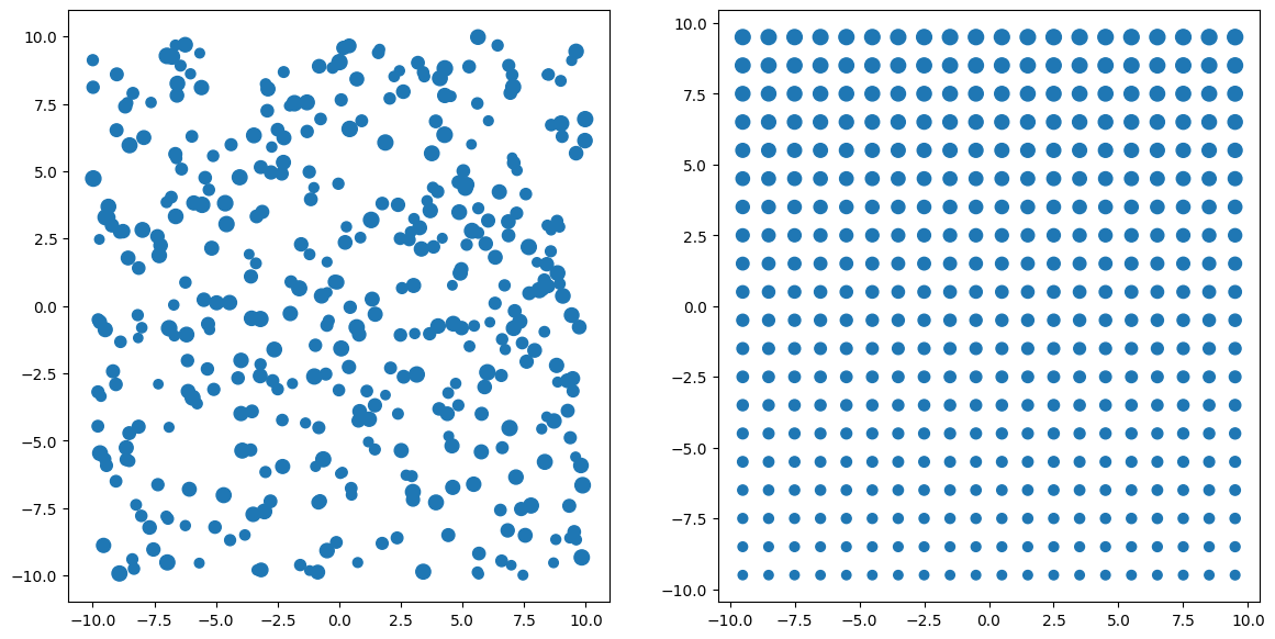
In both cases we generated 400 sources between magnitudes 15 (mmin) and 25 (mmax).
star_field places the stars at random, whereas star_grid place them in a regular partern controled by separation distance.
The size of the simbols illustrate the magnitudes of the stars
Stars#
The core of the stellar module is however the star function which can create any field according to the user needs
In this case we generate a stellar field following a 2D gaussian distribution with a star of every type in the pickles stellar library
from scopesim_templates.stellar import stars
from spextra.database import SpecLibrary

lib = SpecLibrary("pickles")

spectypes = lib.template_names
nstars = len(spectypes)

x = np.random.randn(nstars) * 10
y = np.random.randn(nstars) * 10
mags = np.linspace(10, 20, nstars)

src = stars(filter_name="J", amplitudes=mags, x=x, y=y, spec_types=spectypes, library="pickles")

src.fields
---------------------------------------------------------------------------
ImportError                               Traceback (most recent call last)
Cell In[6], line 2
      1 from scopesim_templates.stellar import stars
----> 2 from spextra.database import SpecLibrary
      4 lib = SpecLibrary("pickles")
      6 spectypes = lib.template_names

ImportError: cannot import name 'SpecLibrary' from 'spextra.database' (/home/docs/checkouts/readthedocs.org/user_builds/scopesim-templates/envs/latest/lib/python3.11/site-packages/spextra/database.py)