Getting Started

scopesim.source.Source objects are composed of a spatial description and a spectral one. Spatial description can be astropy.table.Table objects for point sources or an astropy.fits.ImageHDU for extended sources. Spectral description is provided as synphot.SourceSpectrum or compatible objects. Spectral datacubes can also be accepted

Creation of a Source

The creation of scopesim.source.Source objects might require quite a bit of interaction from the user. For example

import numpy as np
import matplotlib.pyplot as plt
from astropy.io import fits
import synphot
from scopesim import Source

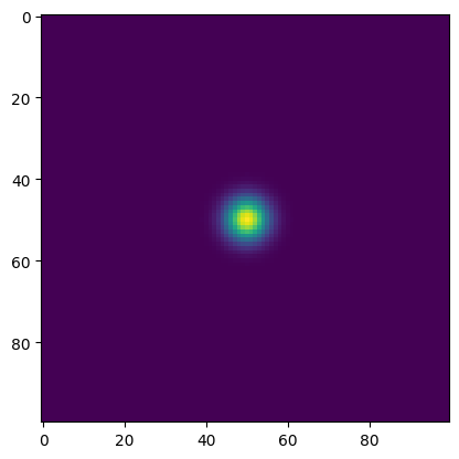
# creation of a image with a central source defined by a 2D gaussian
x, y = np.meshgrid(np.arange(100), np.arange(100))
img = np.exp(-1 * ( ( (x - 50) / 5)**2 + ( (y - 50) / 5)**2 ) )

# Fits headers of the image. Yes it needs a WCS
hdr = fits.Header(dict(NAXIS=2,
                       NAXIS1=img.shape[0]+1,
                       NAXIS2=img.shape[1]+1,
                       CRPIX1=0,
                       CRPIX2=0,
                       CRVAL1=0,
                       CRVAL2=0,
                       CDELT1=0.2/3600,
                       CDELT2=0.2/3600,
                       CUNIT1="DEG",
                       CUNIT2="DEG",
                       CTYPE1='RA---TAN',
                       CTYPE2='DEC--TAN'))

# Creating an ImageHDU object
hdu = fits.ImageHDU(data=img, header=hdr)

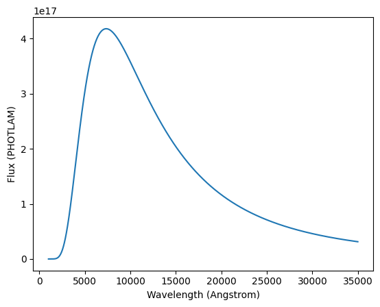
# Creating of a black body spectrum
wave = np.arange(1000, 35000, 10 )
bb = synphot.models.BlackBody1D(temperature=5000)
sp = synphot.SourceSpectrum(synphot.Empirical1D, points=wave, lookup_table=bb(wave))

# Source creation
src1 = Source(image_hdu=hdu, spectra=sp)

plt.imshow(src1.fields[0].data)
src1.spectra[0].plot()

The attributes .fields and .spectra contain the spatial and spectral description of the sources respectively. Datacubes are stored in the cube attribute

These attributes are actually lists of objects which allow to store several sources to be used in one simulation.

Combining sources

For example, let’s create now a simple point source and combine it with the previous one

lam = np.arange(1000, 10000, 1)
flux = np.ones(lam.shape)

src2 = Source(x=[0], y=[0], lam=lam, spectra=flux, weight=[1], ref=[0])

src = src1 + src2

# printing information about the combined source
print(src)

[0]: ImageHDU with size (100, 100), referencing spectrum 0
[1]: Table with 1 rows, referencing spectra {1}

More details can be found in the respective fields

print(src.spectra)

print(src.fields)

[<synphot.spectrum.SourceSpectrum object at 0x7f93b056dd60>, <synphot.spectrum.SourceSpectrum object at 0x7f93d03a1430>]
[<astropy.io.fits.hdu.image.ImageHDU object at 0x7f93b0676b80>, <Table length=1>
   x       y     ref  weight
 arcsec  arcsec
float64 float64 int64 int64
------- ------- ----- ------
    0.0     0.0     1      1]

ScopeSim_Templates

The idea of ScopeSim_Templates is exactly to aid the creation of standard sources to used in the simulator ScopeSim.

Currently the package contain sources to work with stellar and extragalactic objects, as well as general function for other purposes.

The following example combines galaxy and a central source simulating an AGN

from scopesim_templates.extragalactic import galaxy
from scopesim_templates.misc import point_source

gal = galaxy(sed="kc96/s0", amplitude=15, filter_curve="g")  # This will create a galaxy with an S0 SED from the Kinney-Calzetti library (see speXtra)
agn = point_source(sed="agn/qso", amplitude=13, filter_curve="g") # and this an AGN

source = gal + agn

print(repr(source))

[0]: ImageHDU with size (150, 150), referencing spectrum 0
[1]: Table with 1 rows, referencing spectra {1}